Plotting force results

Suppose we are running a force grid search:

ds = grid_search(data, greens, misfit, origins, sources)

After the above command finishes, the data structure ds will contain all the forces and corresponding misfit values.

For a grid of regulary-spaced forces, ds may look something like:

>>> print(ds)

Summary:
  grid shape: (200, 25, 25, 1)
  grid size:  125000
  mean: 2.984e-09
  std:  1.428e-10
  min:  2.605e-09
  max:  3.339e-09

Coordinates:
  * F0          (F0) float64 1e+11 1.012e+11 1.023e+11 ... 9.772e+11 9.886e+11
  * phi         (phi) float64 7.2 21.6 36.0 50.4 ... 309.6 324.0 338.4 352.8
  * h           (h) float64 -0.96 -0.88 -0.8 -0.72 -0.64 ... 0.72 0.8 0.88 0.96
  * origin_idx  (origin_idx) int64 0

Note

Force grids are implemented using parameters F0, phi, h, which are related to r, phi, theta spherical coordinates (physics convention) by F0 = r, phi = phi, h = cos(theta). In addition, F0, phi, h are related to geographic directions by these formulas.

Misfit values

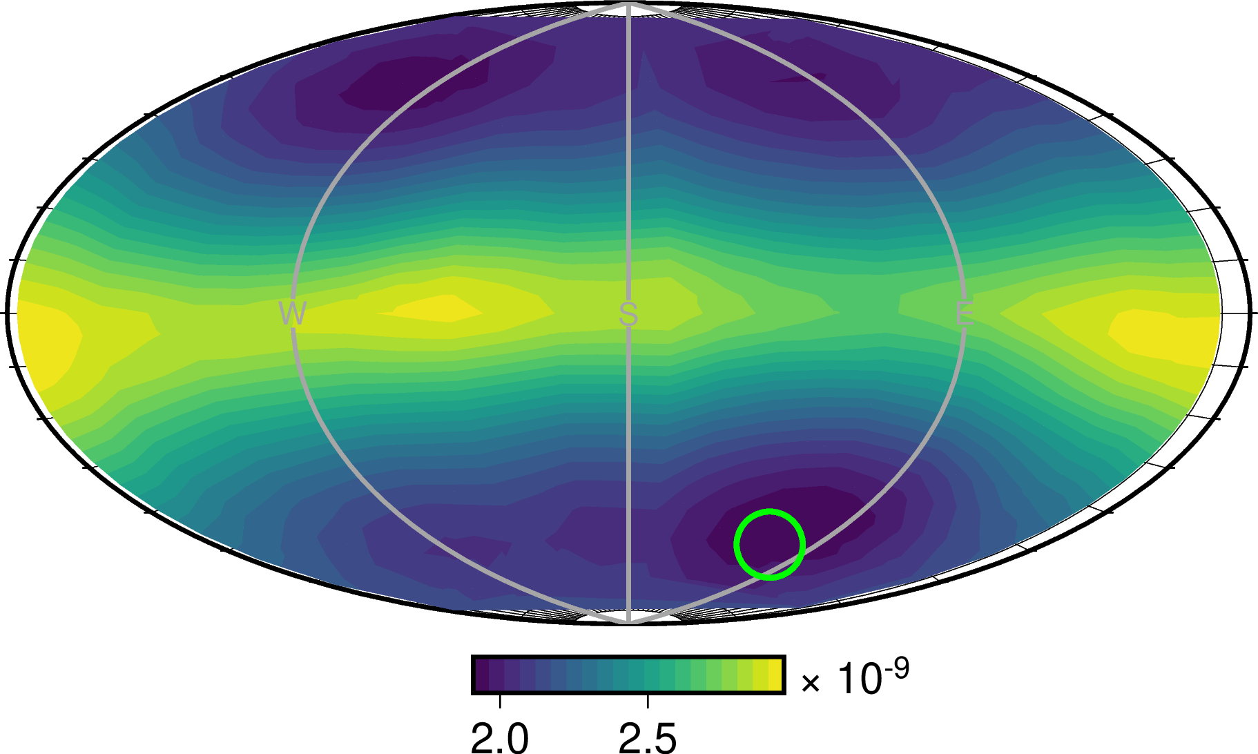
To plot the misfit values returned by the grid search, we can pass ds to a plotting utility as follows:

from mtuq.graphics import plot_misfit_force
plot_misfit_force(filename, ds)

Maximum likelihoods

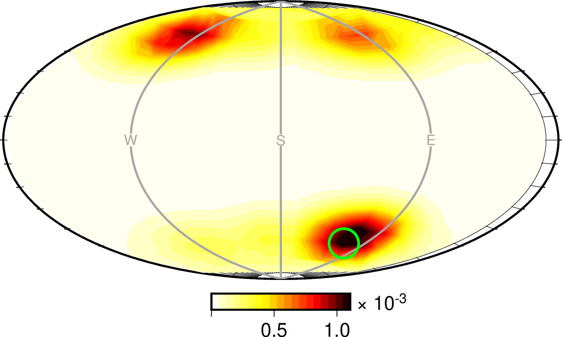
If a data variance estimate var is available, then misfit values can be converted to likelihood values. In the following approach, a two-dimensional likelihood surface is obtained by maximimizing over magnitude:

from mtuq.graphics import plot_likelihood_force
plot_likelihood_force(filename, ds, var)

Tradeoffs between force orientation and magnitude

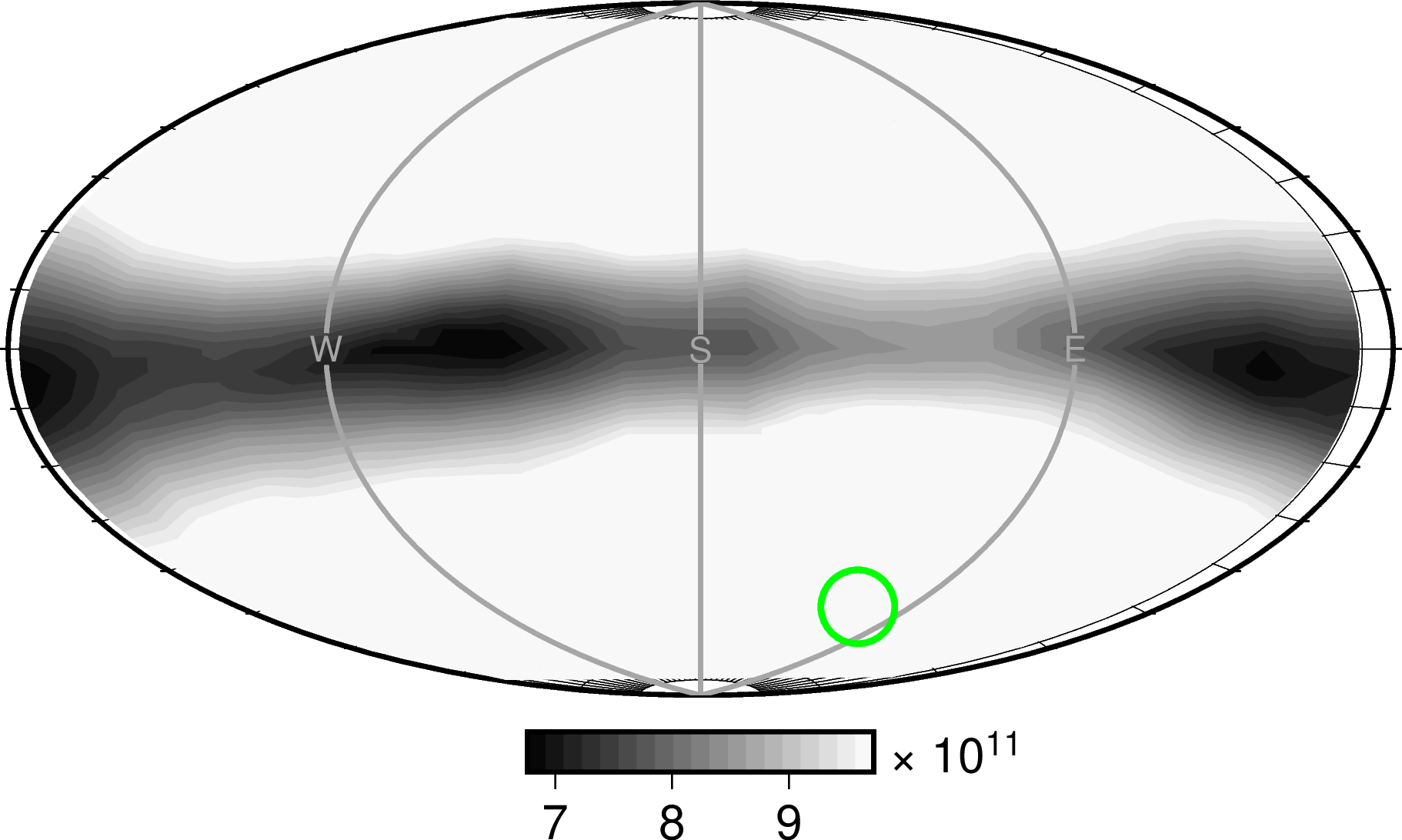
To see how the magnitude of the best-fitting force varies with respect to orientation, we can use the following:

from mtuq.graphics import plot_magnitude_tradeoffs_force
plot_magnitude_tradeoffs_force(filename, ds)

Source code

[script to reproduce above figures]

Users can run the script immediately after installing MTUQ, without any additional setup.