Plotting moment tensor results

Suppose we are running a moment tensor grid search:

ds = grid_search(data, greens, misfit, origins, sources)

After the above command finishes, the data structure ds will hold all the moment tensors and corresponding misfit values.

For a grid of regulary-spaced moment tensors, ds may look something like:

>>> print(ds)

Summary:
  grid shape: (10, 10, 20, 10, 10, 10, 1)
  grid size:  2000000
  mean: 2.548e-09
  std:  2.851e-10
  min:  1.328e-09
  max:  3.640e-09

Coordinates:
  * rho         (rho) float64 5.018e+15 5.418e+15 ... 9.272e+15 1.001e+16
  * v           (v) float64 -0.3313 -0.2995 -0.2371 ... 0.2371 0.2995 0.3313
  * w           (w) float64 -1.178 -1.176 -1.167 -1.141 ... 1.167 1.176 1.178
  * kappa       (kappa) float64 18.0 54.0 90.0 126.0 ... 234.0 270.0 306.0 342.0
  * sigma       (sigma) float64 -81.0 -63.0 -45.0 -27.0 ... 27.0 45.0 63.0 81.0
  * h           (h) float64 0.05 0.15 0.25 0.35 0.45 0.55 0.65 0.75 0.85 0.95
  * origin_idx  (origin_idx) int64 0

Note

Moment tensor grids are implemented using the rho, v, w, kappa, sigma, h parameterization of Tape2012 and Tape2015, from which formulas converting to parameterizations can be derived.

Misfit values

To plot the misfit values returned by the grid search, we can pass ds to a plotting utility as follows:

from mtuq.graphics import plot_misfit_lune
plot_misfit_lune(filename, ds)

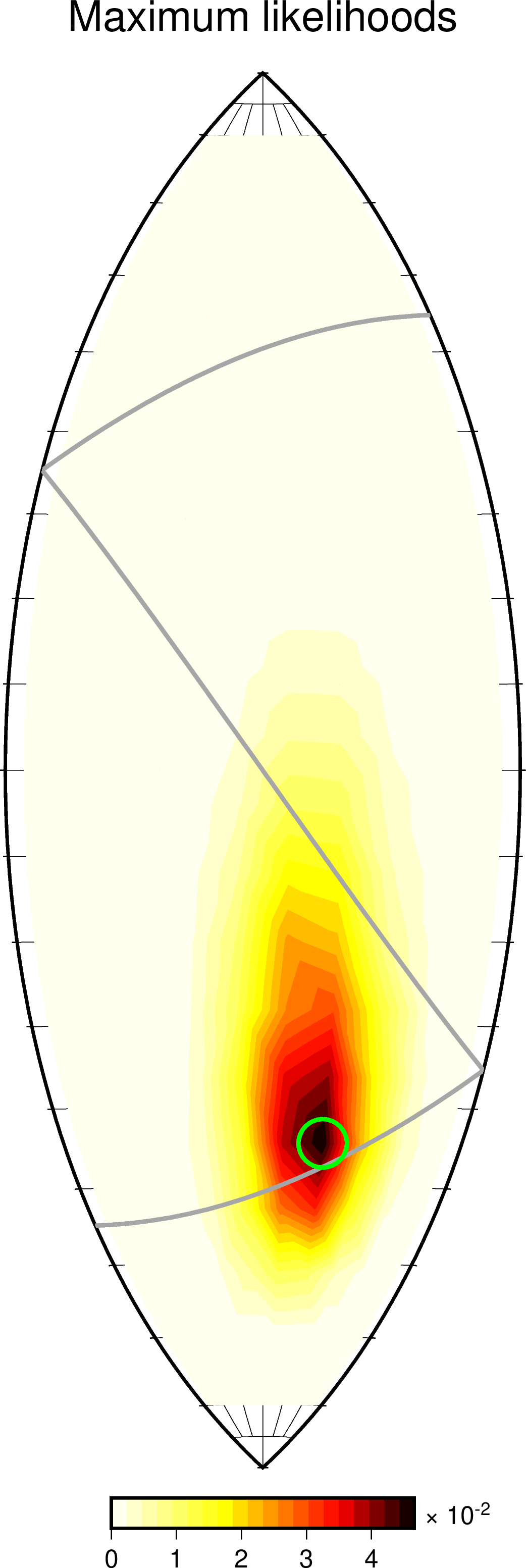
Maximum likelihoods

If a data variance estimate var is available, then misfit values can be converted to likelihood values. In the following approach, a two-dimensional maximum likelihood surface is obtained by maximimizing over orientiation and magnitude parameters:

from mtuq.graphics import plot_likelihood_lune
plot_likelihood_lune(filename, ds, var)

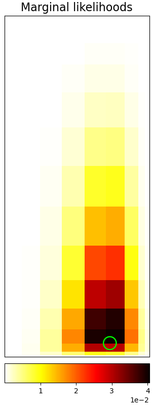
Marginal likelihoods

An alternative for visualizing likelihood is integrate over orientiation and magnitude parameters, giving a two-dimensional marginal distribution. In this case, it is natural to use the so-called v,w parameterization, as follows:

from mtuq.graphics import plot_marginal_vw
plot_marginal_vw(filename, ds, var)

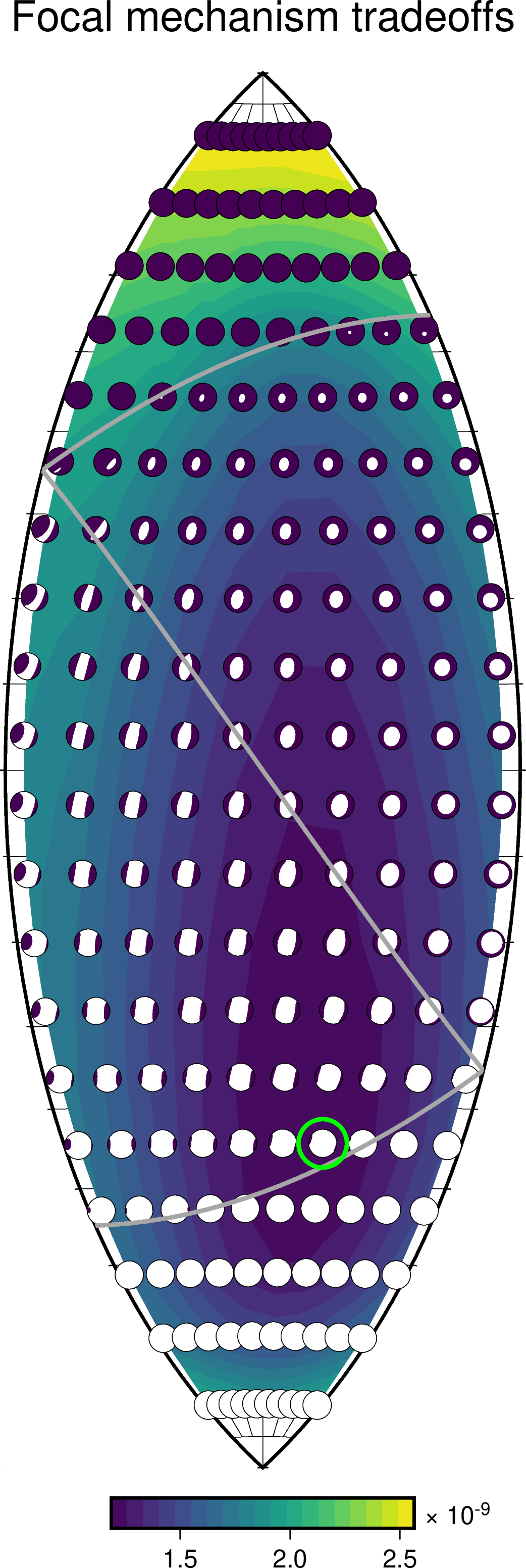
Tradeoffs between source type and orientation

To see how the orientation of the best-fitting moment tensor varies with respect to source type, we can add the show_tradeoffs=True option to any of the plotting utilities as follows:

from mtuq.graphics import plot_misfit_lune
plot_misfit_lune(filename, ds, show_tradeoffs=True)

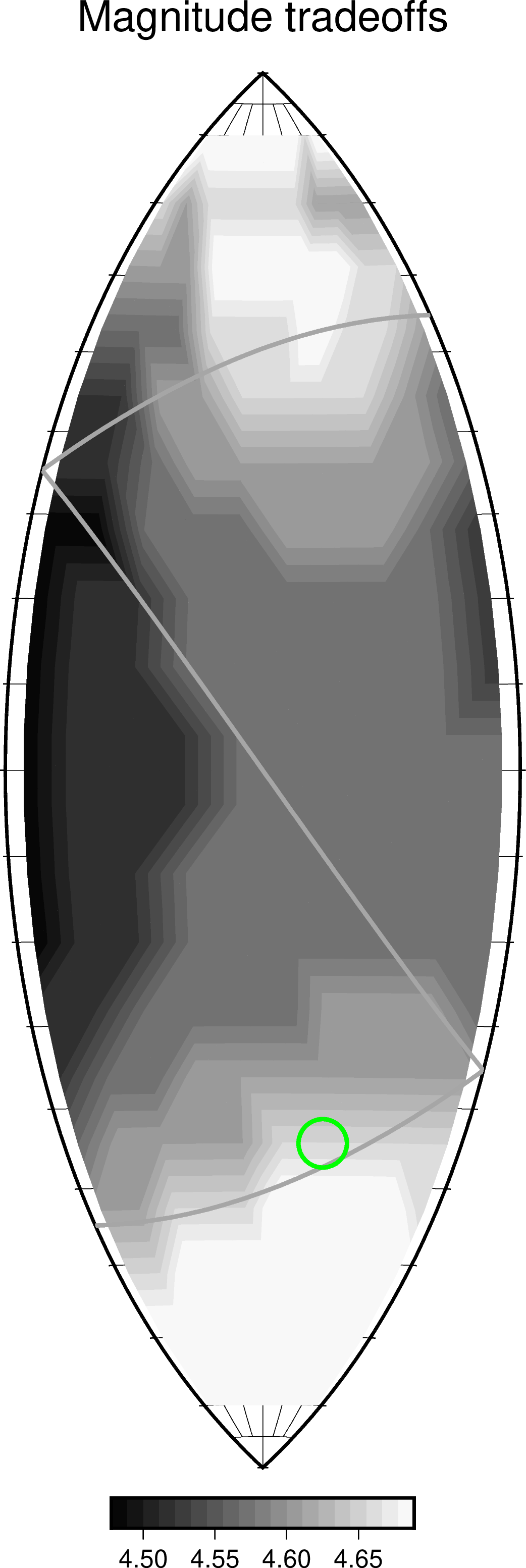
Tradeoffs between source type and magnitude

To see how the magnitude of the best-fitting moment tensor varies with respect to source type, we can use the following:

from mtuq.graphics import plot_magnitude_tradeoffs_lune
plot_magnitude_tradeoffs_lune(filename, ds)

Source code

[script to reproduce above figures]

Users can run the script immediately after installing MTUQ, without any additional setup.